
AutoSpectral: cleaning
- olivertburton

- Oct 27, 2025
- 7 min read
Updated: Mar 25
In this article, we’ll try to cover the functions that AutoSpectral offers for cleaning your single-stained control data.
If you want to follow along with this, you can download the data for this set from Mendeley Data. Alternatively, adapt it to your own samples.
First off, what do we mean by “cleaning”? When we use single-stained cells, they are never really single colour controls. There’s always autofluoresences. This is true for beads in a way–they have background–however with beads, the background is homogeneous (hopefully), whereas with cells we are almost always working with a heterogenous mixtures. That means some cells are more autofluorescent than others, and we can get some cells popping up as “positive” in your data for the fluorophores. AutoSpectral provides some tools to help reduce the influence of these problems, aiming to give you cleaner spectra. Cleaner spectra should lead to more accurate, more precise and more reproducible unmixing.
Right, so there are two main cleaning options in AutoSpectral:
AF exclusion. For this, we need matching unstained samples. AutoSpectral identifies populations of cells with high variance and signal in the unstained sample, and creates a gate around the main trajectory of these cells. It does this by figuring out where the autofluorescent cells are in the unstained and drawing the gate on the main signal of the annoying cells relative to where we expect to see the fluorophore for each control. Cells in the gate are then excluded from the single-stained controls for the purpose of calculating the spectral signatures of the fluorophores. This is on by default because it helps in pretty much all cases, but it's a bit slow at present. It’s not likely to be necessary if you’re running PBMCs or staining other low-AF populations like lymph nodes. Once you get macrophages in the mix (e.g., splenocytes), this can definitely help. AF exclusion is never performed on beads, so as long as your bead samples have been designated as "beads" in the control file (see article), this won't happen on those samples.
Matching negatives. Again, we need matching unstained samples (universal negatives). Here, we’re trying to match the background of the unstained and stained cells as closely as possible. For instance, if we are staining a T cell marker, the correct background to subtract is that of T cells. For a macrophage marker, we want to subtract the background given by unstained macrophages. While we can’t do that perfectly without sorting a whole bunch of different cell types (which wouldn’t work anyway due to changes in cells due to handling), we can do better than just using all the rest of the cells (the internal negative population). If we take the matching unstained sample, we can locate cells that have similar forward (FSC) and side scatter (SSC) profiles and use these as the negative. This works pretty well as long as your negatives and positives have been treated identically and have been run on the same instrument settings. There's probably a more sophisticated way of doing this that would work slightly better, but we're not going to let the best be the enemy of good.
By default, the function clean.controls downsamples the data, selecting the 500 brightest events in the peak channel for each fluorophore’s control. The brightest events are almost always the most accurate, and this speeds up the calculations a great deal. Better results, faster.
Okay, let’s go over some data as an example.
We need to set up our experiment. This is Aurora data. See the control file and gating articles for more info.
asp <- get.autospectral.param( cytometer = "aurora", figures = TRUE )
# optional: turn on parallel processing
asp$parallel <- TRUE

# where are the single-stained controls?
control.dir <- "./SSC"

# create an initial file detailing the controls
# this requires manual editing
create.control.file( control.dir, asp )

# splenocyte controls for everything
control.file.cells <- "fcs_control_file_cells.csv"

# For this set, we need to expand the large gate parameters
# more on this in the gating article
asp$large.gate.scaling.x <- 3
asp$large.gate.scaling.y <- 6
flow.control.cells <- define.flow.control( control.dir, control.file.cells, asp )

We can get the fluorophore spectra using only the Robust Linear Modelling approach (no cleaning). This is slow since it calculates over all the gated data (no downsampling).
spectra.cells.rlm <- get.fluorophore.spectra( flow.control.cells, asp,
                                              title = "Cells RLM" )
See those horizontal lines? That’s the autofluorescence “dirt” in the controls. An autofluorescence spectrum is across the bottom and there’s some similarity.

Keep an eye on that mixing matrix condition number as we progress through the cleaning steps. The condition number more or less tells you how much trouble you'll have unmixing the data (lower is better).
It’s recommended to at least do the first cleaning step: setting universal negatives. This restricts the calculations to the brightest events plus scatter-matched negative events from the universal negative. This speeds things up considerably.
Note that when you call clean.controls, it outputs a copy of your flow.control structure with a new set of data that is just the “clean” events. It still has the original “dirty” data. This means you can overwrite the flow.control if you want, which reduces memory usage.
clean.control.cells.neg <- clean.controls( flow.control.cells, asp,
                                           universal.negative = TRUE )
# or:
# flow.control.cells <- clean.controls( flow.control.cells, asp,
#                                           universal.negative = TRUE )
See folder figure_scatter and figure_spectral_ribbon for plots.
Selected CD64-positive events (macrophages) and matching negative region:

The same for CD8 (T cells):

It isn’t always easy to see the impact of this, but if we look at the cells with a higher average level of autofluorescence, like myeloid cells, we can usually spot it. In the spectral ribbon plot below, we’ve got the distribution of signals for the selected negative events (top row), brightest positive events (middle) and the bottom row is the difference between the two (background-subtracted). In this case, it’s CD11b and the brightest tend to be neutrophils. You can see how the middle violet area is up in the top and middle rows and that this mostly gets cancelled out in the bottom row.

Note that we’re displaying all the data here. On the Cytek Aurora, there’s some sort of cut-off in SpectroFlo software so you don’t see the low frequency tails of the distributions. This makes it look like the data is better than it actually is.
We can now extract the spectra again, using the cleaned data (use.clean.expr = TRUE).
spectra.cells.neg <- get.fluorophore.spectra(
 clean.control.cells.neg,
 asp,
 use.clean.expr = TRUE,
 title = "Cells Matching Negative"
)
Did this help? Yes, there are a couple of fluorophores that are now not just streaks of yellow across the board.
To see what’s changed, we can subtract the cleaned spectra from the original RLM spectra.
delta.cells.rlm.neg <- spectra.cells.rlm - spectra.cells.negWe can create a heatmap (see Plotting article) to visualize this (this function still needs some work, sorry).
create.heatmap( t( delta.cells.rlm.neg ),
                legend.label = "Change in spectra",
                title = "Matched negative change cells",
                output.dir = "./figure_spectral_change" )
The other recommended cleaning step that is recommended is to use af.remove to exclude intrusive autofluorescent events from the spectral calculations. We’ll use the scatter-matching negatives and brightest event selection as well.
clean.control.cells.af <- clean.controls( flow.control.cells, asp,
                                          universal.negative = TRUE,
                                          af.remove = TRUE )
See figure_clean_controls for plots.
The Siglec F BUV615 single-stained control is a nice example here. This marker is present on eosinophils, a little bit on mast cells and on alveolar macrophages, none of which is present to any great extent in C57BL/6J mouse spleens under SPF conditions. There is, however, quite a bit of noisy autofluorescence in that part of the spectrum.
Here’s the matching unstained sample, which we use to define the gate around the region of intrusive autofluorescence noise. This gate is drawn on one of the high AF channels (V7-A in this case) versus the expected peak for the fluorophore (UV10-A in the case of BUV615 on the Aurora).
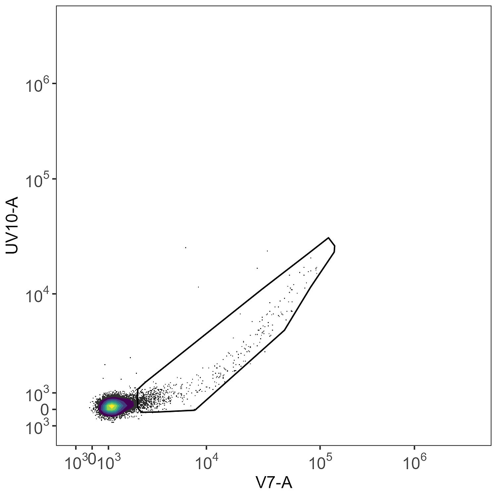
We then copy this gate to the BUV615 single-stained control. Notice how the intrusive AF events are in the same place, but we now have a (very small bit of) signal in the UV10-A channel that wasn’t there before. That’s the very few, dim cells we’re trying to use to define the BUV615 signature. This signal would be completely overwhelmed by the AF noise, and if you look at the spectral heatmaps up above you’ll see that the BUV615 line is quite yellow with a large signal in V7. Making sense now?

Of course, a good solution might be to use compensation beads for controls like this. BUV615, unfortunately, is one of those dyes that doesn’t do so well with beads.
We also get spectral ribbon plots, this time to show us what the data look like with and without the removal process in place. You’ll want to check these because they'll help you appreciate what's going on.

This is one of the parts I really like. We get the original data across the top, which is honestly just a bunch of noise. With the cleaned data in the middle, though, we can start to pick out the two expected peaks for BUV615: middle UV (UV10) and narrow YG (YG3). It’s just a hint, but it’s there. And across the bottom, the junk we’re excluding, which is basically a bunch of macrophages getting in the way.
We can now extract the spectra using the cleaned data without AF events.
spectra.cells.af <- get.fluorophore.spectra( clean.control.cells.af, asp,
                                             use.clean.expr = TRUE,
                                             title = "Cells AF Removed" )

Remember where we started with the condition number? It was over 80. Same panel, same controls, different result.
What has changed with this cleaning procedure?
delta.cells.rlm.af <- spectra.cells.rlm - spectra.cells.af
create.heatmap( t( delta.cells.rlm.af ),
                legend.label = "Change in spectra",
                title = "AF removal change cells",
                output.dir = "./figure_spectral_change" )


Comments