Data Analysis in Honeychrome: Honeycluster

olivertburton

23 hours ago

9 min read

Updated: 6 hours ago

Today's post will try to give an overview of how to use one of the data analysis workflows in the free open-source Honeychrome app. This first, one, called Honeycluster, is a basic dimensionality reduction and clustering workflow, but with some statistical tools added to help you sort out the biological meaning from your results. The aim is to provide an end-to-end workflow, incorporating optimized unmixing, automated autofluorescence extraction, automated transformation settings, robust statistical analysis and publication-ready plotting.

This is new, and there are definitely some missing features (batch correction, multi-experiment analysis), and probably some bugs I haven't found yet. I also want to make clear that this is not something new, just a knitting together of existing analysis approaches, and that this is based on the work of many people. I'll put some references at the end, but you can also visit the further reading page to learn about the techniques used in Honeycluster. Furthermore, you can find similar workflows, for free, as detailed in this post. A lot of effort has been put into those existing pipelines, including trying to make them easy to use and interact with.

In Honeychrome, you'd start by performing your unmixing first. See this post for how to do that, and also check out the help pages on the Honeychrome website.

For today's post, I'm going to be using some data from a few years ago, testing the importance of the transcription factor BATF for regulatory T cell homeostasis in various tissues through the body. You can download the data and the .kit file for Honeychrome from this repository on Mendeley. The data are from a Treg-focused panel for the Aurora (a bit old and not great by today's standards), and the key thing to know is that we will be comparing the CD45.1- (CD45.2) cells, which are either BATF-KO or WT, depending on the mouse. (We aren't doing the comparison within the same mouse between CD45.1 and CD45.2 in part because CD45.1 mice have polymorphisms that affect immune cells and largely because the released version of Honeychrome doesn't have that capability built in yet. That will go into the next release.)

Once the unmixing is done, move to the Unmixed Data tab and set up your gating strategy. Here, I've just set up a couple of simple gates for viable lymphocytes, T cells, CD4/CD8 and Tregs as CD3+CD4+Foxp3+.

The data analysis modules are plugins. This means they aren't shown by default, and you'll need to turn them on. Go to the Edit menu and select "App Configuration".

Scroll down to where you see "Bundled plugin" and tick the box for Honeycluster:

Hit OK. The app will refresh, so the main window with close and reopen (probably at a different size than it was, something to fix).

Now, you should have a Honeycluster tab appear. Click on it and you should see this:

The layout here:

On the left, the samples, arranged as we have them in folder in the experiment folder.
The column with Transforms, Configuration, etc., contains the elements you'll go through for the Honeycluster workflow, top to bottom.
In the middle, we have the gating hierarchy, and we can select which populations to display. I've selected T cells.
We then have a 1D histogram and a 2D biplot (currently empty) to display the data so we can evaluate the transformation settings.
On the right, the list of channels we have available for this data. We can select the displayed x-axis on the plots by clicking on the plot label or by selecting from the list on the right.

Transforms

To view some data, click on a sample. I'll use a spleen sample.

The first step for dimensionality reduction and clustering is to scale the data, setting appropriate transformations. Honeychrome uses a logicle (read: biexponential) scale, like you're used to from the cytometer. When you start, the transformations will be whatever is set in the Unmixed Data tab, which will be a default transformation setting for the cytometer you're using or whatever you modified them to be. You can adjust the transformation for any channel by dragging on the axis. Dragging on the lower half affects the compression around zero (the width basis), and dragging on the upper half changes the range (the maximum displayed value).

For instance, starting here:

Dragging around zero to make the negative smaller:

Dragging up from 10^5 to make CXCR3 take up more of the viewed space:

These sorts of changes affect how the clustering and dimensionality reduction algorithms "see" the data, much the way they affect our perception of it. To make things easy, Honeycluster has an automated option to adjust the width basis, based on a slight modification of the recommended approach in the original publication on the biexponential/logicle transform. To use it, hit the "Auto-transform" button.

You get a popup when it finishes, telling you what it has done. The result in this case looks like this:

Pretty much everything should be visible on the plot, and the negative population should be fairly compact. If you don't like it, you can override manually or use the "Reload from experiment" button to go back to what you had in the Unmixed Data tab. The transformation settings in the Honeycluster analysis plugin don't carry over to the Unmixed Data tab.

Configuration

The configuration tab is where we set up our clustering and dimensionality reduction runs.

Data selection

At this point, the sample column on the left disappears because we don't need it anymore.

In this tab, we select the gate we want to use (which cells), the parameters we want to analyze (which markers), how many cells to use and which samples we want to include. I've selected my T cells, all of the markers that I haven't already used for gating to get to those cells, 5000 events per sample (or as many as it has if it there are fewer than 5000), and I'm running liver, mesenteric lymph node (MLN), spleen and axillary lymph node (LN).

Dimensionality Reduction

Click the "Dimensionality Reduction" flap to open it. We can choose between UMAP, tSNE and PaCMAP. There are some parameters you can modify if you want, but generally the defaults are pretty good. If you want to learn more about anything, click the "Show Help" button.

Let's do a UMAP. I have a "Trained" message in green because I've already run one.

Now, because dimensionality reduction and clustering can take a long time if you have a lot of data (or a slow computer), the first thing that happens is we estimate how long it's going to take:

You then get a popup telling you about how long it will take and asking you to confirm you want to go ahead. This estimate will get more accurate as you run this more on your computer.

It's going to take about a minute and a half. Let's do it. You can also cancel mid-run if you need to.

Once it's done, we get this "Trained" message:

And the run is stored in our Archive (bottom subtab):

Here you can edit the Label to be something more meaningful to you.

Same thing for clustering. Options are FlowSOM, Leiden (Phenograph-ish) and HDBSCAN. Leiden and HDBSCAN try to figure out how many clusters you have; for FlowSOM, you need to decide how many to look for.

For FlowSOM, you generally won't see a timing estimate popup. It would take longer to time it and dismiss the message than to just run the clustering. Note: we probably need more than 10 clusters here.

One point: you can cluster on either the original features (your high dimensional flow data) or the embedded space (the tSNE or UMAP coordinates). In the flow field, people mostly cluster on the original features, which can sort of give some idea of how well the algorithms agree on the data. This is an area where people tend to have strong opinions, and I guess mine is that clustering and dimensionality reduction just isn't a great method for analyzing flow cytometry data. Anyway...

Cluster Annotation

Once you have a bunch of clusters, you've got to figure out what they are. This tends to be the limiting factor in the analysis, and there's some work going on in this area (e.g., SOULCAP, CellScope.ai). This problem exists because we've through out the baby with the bathwater. Anyway...

To help you figure out what you've got, Honeycluster provides lots of plots and a couple of annotation tools. In the Cluster Annotation tab, select the clustering run you want (if you have more than one), and pick the channels you want to see plotted.

Under "Clustering run:", where it says "Annotation", we can also toggle over to "Marker Heatmap/Ridgelines". This will take a few seconds to load (more clusters, more time). This shows you another way of viewing the marker expression levels per cluster.

Back in the "Annotation" part, we can see how our clusters fit onto our dimensionality reduction embedding.

If you have run different algorithms, toggle between them using the "DR run" dropdown.

At the bottom, we have a table with our clusters, where we can change the name and colours associated with them.

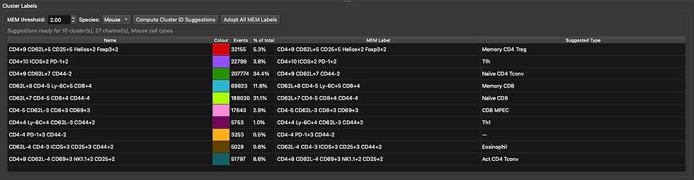
We can also run Marker-Enrichment Modelling (MEM) and a very simple and not amazing matching to cell types based on scType. Perhaps these are helpful. Click "Compute Cluster ID Suggestions" after setting the species correctly. I get a popup with this data saying that TNFRII wasn't recognised (not in the database yet), and that it did not contribute to the scoring.

Is that correct? Not entirely, no. We don't have eosinophils--these are T cells. Maybe it helps, though. This will be a little better in the next release.

The MEM scores are descriptive, so they are always correct, just maybe not what we want. For now, I'm just going to use those, since that's better than Cluster 0-9. Hit "Adopt All MEM Labels" to do that. You'll get a popup where the default is "No", so hit "Yes" to confirm.

Stats

This is probably the most important part of the workflow because it allows to ask questions of the data. Hopefully the help text is clear enough to follow.

The table at the top is where we define what our experimental groups are. I've created BATFKO and WT groups. Those will be the labels on the analysis. They can also match to the filenames to sort the samples into the appropriate groups. Alternatively, you can use the "Match pattern (regex)" to gather samples into groups. For instance, if I'd put "mutatnt" in the file name instead of BATF, I could use BATF as the group label and mutatnt as the matching pattern.

To use the regex matching, fill in the "Match pattern" and hit "Auto-assign by pattern" to fill in the table below for the samples.

Alternatively, use the "Suggest Groupings..." button.

This detects repeated elements in the file names and suggests them as grouping variables. Here it has picked up BATFKO and WT as the biggest distinction, tissue as another, and the other three fields are the mouse identifier elements. You can change the name of a column/group, for example, "field_1" I would rename as "Tissue". Click Apply to use it.

You can also manually add and remove columns using the corresponding buttons, or import a CSV file that you may already have prepared in the same layout.

Scroll down to "Differential statistics" below this table. Select the clustering run you want to analyse. Select the groups you want to compare, and any variables you want to adjust for or use for pairing. I'm measuring the effect of BATF, adjusting for tissue as a covariate.

Scrolling down, select whether to test cluster frequencies, cell counts and/or MFIs. You can configure which markers are tested. Note: for MFIs, this is a "cluster-first" approach, so only clusters that shift statistically based on frequencies/counts will be tested for MFI changes, mostly to avoid producing overwhelming amounts of information. Click Run Statistics.

Results

We can view the distribution of clusters on a per-sample level on a PCA, with the loadings (arrows) telling us which factors are shifting along each vector.

Volcano plot showing changes in cluster frequency

Heatmap of statistically significant clusters

Volcano plot of MFI changes on differentially abundant clusters

Right-click on a point in a volcano plot to show the distribution between groups:

Layout

Here you can add plots to the page to make a presentation of your data. I think this should be fairly self-explanatory, and there's also a help button if you get lost. Change the "Theme" button to toggle between light and dark backgrounds.

Report

Create a report containing anything you want from the analysis you've run. It will be compiled into a PDF and you'll also get individual image files, which you can arrange as you like in other software. You also get CSV files, so you can re-run the analysis elsewhere if you prefer. Everything goes into the folder for the experiment, in Honeycluster Reports.

References:

A new "Logicle" display method avoids deceptive effects of logarithmic scaling for low signals and compensated data (Parks, Roederer and Moore 2006, Cytometry A)
FlowSOM (Van Gassen et al. 2015, Cytometry A).
Analyzing high-dimensional cytometry data using FlowSOM (Nature Protocols)
Phenograph (Levine et al. 2015, Cell). Picks out how many clusters there "should" be. See also the blog post: https://www.colibri-cytometry.com/post/the-peculiarities-of-phenograph
Leiden (Traag, Waltman and van Eck 2019, Scientific Reports): Improves on the Louvain algorithm used in the original Phenograph.
HDBSCAN (Campello, Moulavi and Sander 2013, PAKDD): Density-based, with a noise label. Also automatically determines cluster number.
MEM, marker enrichment modeling (Diggins et al. 2017, Nature Methods):
ScType (Ianevski, Giri and Aittokallio 2022, Nature Communications):
Cellscope A fee-for-service platform that provides cluster annotation for flow cytometry data.
limma (Ritchie et al. 2015, Nucleic Acids Research)
Linear models and empirical Bayes methods (Smyth 2004, Stat Appl Genet Mol Biol)
TREAT: testing relative to a threshold (McCarthy and Smyth 2009, Bioinformatics)
Selective inference on multiple families of hypotheses (Benjamini and Bogomolov 2014, J R Stat Soc B)
edgeR (Robinson, McCarthy and Smyth 2009, Bioinformatics): Negative-binomial models for counts.
diffcyt (Weber et al. 2019, Communications Biology)
The ASA statement on p-values (Wasserstein and Lazar 2016, The American Statistician)
Statistical errors (Nuzzo 2014, Nature)
The new statistics and a Bayesian alternative (Kruschke and Liddell 2018, Psychon Bull Rev)
How to prepare spectral flow cytometry datasets for high dimensional data analysis
Fast interpolation-based t-SNE for improved visualization of single-cell RNA-seq data (Linderman et al. 2019, Nature Methods)
PaCMAP: Understanding how dimension reduction tools work (Wang et al. 2021, JMLR)