
Predicting unmixing errors
- olivertburton

- May 20
- 5 min read
Today’s post is a bit more speculative. This means I'm probably wrong about some of it, so chime in to correct me. I thought I'd share this information anyway because it is as accurate as I can make it at present and it appears to be useful.
Edit: This pre-print is hitting on the same idea, I believe, using the variance-covariance structure to predict spread:
One key problem in spectral cytometry is what to do when the unmixing isn’t correct. An important step towards fixing this is being able to determine when we have errors and where they are coming from. I've done a bit of work on this implicitly in AutoSpectral, but today I'm going to try to lay out the theory behind that. Fortunately, there appears to be a bunch of well-known mathematics from the field of statistics that concords with the intuition I had on this (at least, if I understand the mathematics correctly, which I may not).
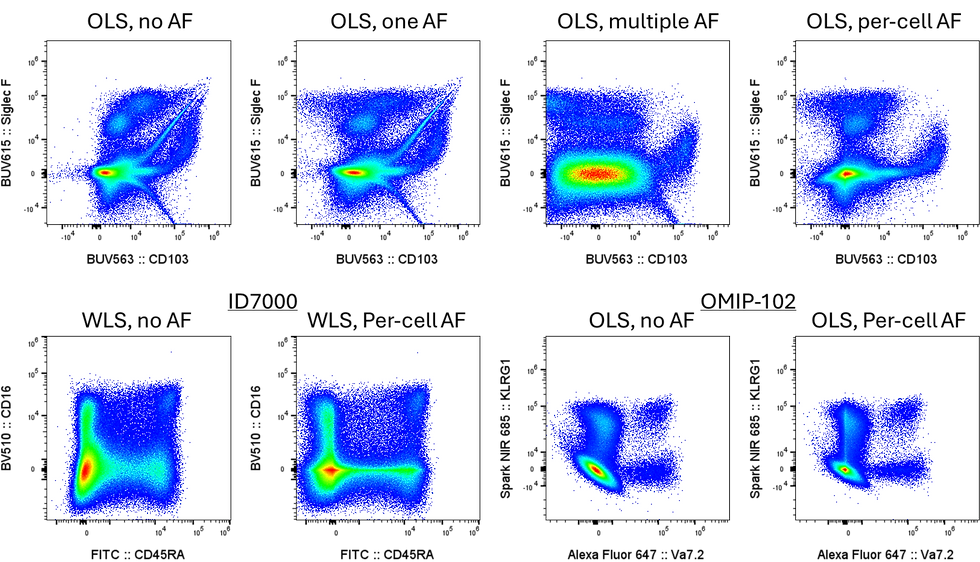
Let’s consider an example of tandem breakdown as a thought experiment for producing an unmixing error with a known source. We stain with something like PE-Cy7, we have a single-stained control and some multi-color samples. Let’s suppose we make our control quickly using beads, chucked it in the fridge, then spent an hour making our master mix for the samples on the bench in the light. We now have a big discrepancy in light exposure, which will result in differential tandem breakdown between the control and the samples. Specifically, we will get more breakdown on the samples, so more PE-like signal. If we have PE as well as PE-Cy7 in our panel, we will get unmixing error, skewing the PE-Cy7+ cells towards PE. (For tips on tandem handling, see this article and this one.)
Now, if we look at our unmixed data, how do we know there is an unmixing error? In this example, there is undeniably more PE signal because we have created more PE without the Cy7 attached. It’s just that some of the PE was originally PE-Cy7. Most experienced cytometrists could probably tell you from looking at a plot of this data that there’s tandem breakdown going on, though, so the information is there. Could we tell where the error was going to occur ahead of time, though, without prior knowledge of the biology? I think the answer is yes, and not just for this trivial example.
One of the things AutoSpectral does is measure the variability in the spectral profiles present in your single stained control samples (Ozette's Resolve also appears to do this). That variation in fluorescence stems from a lot of factors, too many to go into here. The point is, there isn't just one outcome, but rather a distribution of possibilities. We can show that variability as a bunch of overlaid profile traces:

If we plot the variation as the standard deviation of the values in each detector, we are effectively looking at a map of where this fluorophore is variable:

Notice where the red is? There's a bunch in YG-1 (PE peak channel) and in YG10, where the longer wavelength photons have a long tail of emission. We then get echoes of this pattern across the other lasers since PE is so good at catching photons.
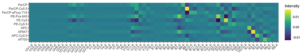
We can combine all of those standard deviations of the variability for all the fluorophores in the panel into a heatmap:

Now we are getting close. This is just summarizing the variability in the raw detector space, though. We want to know about the error in the unmixed data space. This variation in the raw space is our measurement error. It propagates into the unmixed space. How? Through the unmixing matrix.

This is our error propagation in the unmixed space. In other words, this should be a map of where we should look for unmixing problems, both skewing and spreading. Read across the rows to understand how a fluorophore will impact on others. A couple examples: PE-Vio770 (our PE-Cy7-like dye) has a yellowish square versus Spark YG 570 (a PE replacement) and a bright yellow square versus PE-Fire 810. BUV661 has a bright spot versus APC (it causes lots of spillover spread into APC). PerCP-eFluor 710 has a bright spot versus every ~700nm emitting dye because PerCP gets excited a lot, by everything. As with all things, the total error you observe will be proportional to the amount of signal you have; this does not account for that.
What are we saying here? We have some error (variability) in our measurement of the raw data. That error doesn't necessarily go away when we unmix the data. It gets better or worse depending on what your unmixing matrix looks like. The variability will matter if you have other fluorophores that are collinear with (similar to) that variability (not the dye's signature itself). If you are working with PerCP-Cy5.5, and hopefully you are not, the massive variability that dye produces will matter if you have other dyes in the many, many regions where PerCP-Cy5.5 is variable, but will not matter if you're only use PerCP-Cy5.5 and BUV395 because the variability essentially cannot be collinear. If you have a fluorophore that varies in the red laser detectors, you will likely see variability (spillover spread) versus fluorophores that are relying on the red laser detectors for unmixing (i.e., dyes with peaks on the red laser detectors). So, BUV661 -> APC. If your measurement of the center of the distribution of fluorophore profiles (the nominal spectrum) for a given fluorophore is off (a bad control, badly extracted signature, sample treated differently), you will get a skew, AKA an unmixing error, and you will probably get it in the same areas where the variability is collinear with the nominal spectrum for other dyes because that is where the uncertainty lies. To the best of my understanding, this does not tell us the direction of any skew, just where it's likely to happen.
Anyway, that is the basic concept. In statistics, it appears to be the convention to use the standard deviation except when the variables are correlated. I think it may be better to use the covariance in the case of flow cytometry because we have multiple laser excitation events, which means the changes in emission tend to be linked (more direct excitation of the FRET acceptor tends to go with less full tandem signal). In the example here, that makes little difference, but it has more impact when dealing with more highly variable signals like autofluorescence.

What AutoSpectral does is it tries to calculate where each cell lies on the distribution of variability for each fluorophore and also the autofluorescence. By setting each cell's unmixing matrix to use those calculated positions, we "center" the cell in the distribution across all parameters (in an ideal world), bringing it closer to true and reducing some of the uncertainty and error. For that to work, though, we need good controls, because we are making them work a lot harder.
What AutoSpectral does not do is any sort of Monte Carlo iteration or Bayesian inference to get a better estimation of the error propagation. That would probably give better unmixing.


Comments